


Every day, software makes thousands of yes or no decisions. A bank decides whether to approve a loan. An email service decides whether a message is spam. A hospital system flags whether a patient faces a high risk. Behind many of these choices sits one simple and powerful method: logistic regression.
Logistic regression predicts the probability of a category. It takes numbers as input and returns a value between zero and one. You then turn that value into a class, such as yes or no, spam or safe, buy or leave.
This guide explains logistic regression from the ground up. You will learn the math, the main types, and the code. You will see how logistic regression compares with linear regression. You will also see how researchers and engineers apply logistic regression in real projects.
What is logistic regression?
Logistic regression is a supervised learning method for classification. It studies the link between one or more input variables and a categorical outcome. The outcome usually has two values, such as pass or fail. The inputs can be numbers or categories.
The name confuses many beginners. The word regression suggests that the model predicts a number. In practice, the model predicts a probability, and you use that probability to assign a class. So logistic regression works as a classifier, even though it carries the regression label.
The key idea in plain words
Imagine you want to predict whether a student will pass an exam. You know how many hours the student studied. More hours usually mean a higher chance of success. A straight line cannot model this chance well, because a line keeps going up and can cross one. A probability can never exceed one.
Logistic regression solves this problem with a smooth S shaped curve. The curve starts near zero, rises slowly, climbs fast in the middle, and flattens near one. Every input maps to a point on this curve. That point is the predicted probability.
Why the S curve matters
The S curve keeps every prediction between zero and one. It also behaves in a sensible way. Small changes in the input cause small changes in probability at the extremes. They cause bigger changes near the middle, where the model feels unsure.
Analysts call this curve the sigmoid function or the logistic function. The method takes its name from this function. The next section shows the exact formula.
Core terms you should know
- Dependent variable: the outcome you want to predict, such as default or no default.
- Independent variables: the predictors, such as income, age, or hours studied.
- Coefficient: a number that shows how strongly a predictor pushes the outcome.
- Odds: the chance an event happens divided by the chance it does not happen.
- Decision threshold: the cutoff that turns a probability into a class label.
Logistic regression formula
The math behind this model has three parts. First, the model builds a linear score. Second, it converts the score into a probability. Third, it learns the best coefficients from data. Let us walk through each part.
Step one: the linear score
The model starts like linear regression. It multiplies each input by a coefficient and adds the results. It also adds a constant called the intercept.
z = b0 + b1x1 + b2x2 + … + bnxn
Here, b0 is the intercept. Each b value is a coefficient. Each x value is a predictor. The score z can take any value on the number line, from very negative to very positive.
Step two: the sigmoid function
Next, the model squeezes the score into a probability with the sigmoid function.
p = 1 / (1 + e to the power of negative z)
The letter e is a mathematical constant, about 2.718. When z equals zero, p equals 0.5. When z grows large, p moves toward one. When z becomes very negative, p moves toward zero.
Step three: odds and log odds
The formula has a second view that analysts love. Start with the odds, which equal p divided by (1 minus p). Then take the natural log of the odds. That value equals the linear score z.
ln(p / (1 minus p)) = b0 + b1x1 + b2x2 + … + bnxn
This form explains the model neatly. The log odds change in a straight line as the inputs change. The probability itself follows the S curve.
This view also explains the coefficients. When x1 rises by one unit, the log odds rise by b1. If you raise e to the power of b1, you get the odds ratio. An odds ratio of 1.5 means the odds grow by 50 percent for each extra unit of x1. An odds ratio below 1 means the odds shrink.
How the model learns the coefficients
Linear regression uses least squares. This model uses maximum likelihood estimation instead. The method searches for the coefficients that make the observed data most likely.
In practice, the algorithm minimizes a cost function called log loss, or binary cross entropy. For one observation, the loss grows large when the model gives a low probability to the true class. It stays small when the model gives a high probability to the true class. The algorithm adds the loss across all rows and tries to shrink the total.
Gradient descent in simple terms
No closed form solution exists for the best coefficients. So the computer uses an iterative search. Gradient descent is the most common choice.
The steps look like this:
- Start with small random coefficients, or with zeros.
- Predict a probability for every row.
- Measure the error between each prediction and the true label.
- Adjust each coefficient a little in the direction that reduces the error.
- Repeat until the loss stops improving.
The size of each adjustment depends on the learning rate. A tiny rate learns slowly. A huge rate overshoots and never settles. Libraries such as scikit learn use faster solvers, but the idea stays the same.
Logistic regression types

Not every classification task has two outcomes. Because of that, analysts use three main versions of this model. Each version fits a different kind of target variable.
Binary logistic regression
Binary logistic regression handles two outcomes. Examples include fraud or not fraud, churn or stay, and disease or healthy. This version is the most popular one. When people say logistic regression without any label, they usually mean the binary case.
Multinomial logistic regression
Multinomial logistic regression handles three or more outcomes with no natural order. Think about predicting a customer’s favorite product category: books, music, or games. The model estimates one probability for each class. All probabilities add up to one. The class with the highest probability wins.
Many libraries use the softmax function here. Softmax extends the sigmoid idea to many classes. Another approach, called one versus rest, trains one binary model per class and picks the strongest result.
Ordinal logistic regression
Ordinal logistic regression handles outcomes that have a natural order. Survey ratings such as poor, fair, good, and excellent fit this pattern. The model respects the order and uses cumulative probabilities. It needs fewer parameters than a multinomial model and keeps the ranking information.
Quick comparison
| Type | Outcome | Example |
| Binary | Two classes | Spam or not spam |
| Multinomial | Three or more classes, no order | Product category |
| Ordinal | Three or more classes, ordered | Satisfaction rating |
Choose the version that matches your target. If you force an ordered outcome into a multinomial model, you lose useful information. If you force a multi class outcome into a binary model, you hide important differences.
Learn more……..Image Recognition: How Machines Learn to See and Understand Pictures
Logistic regression vs linear regression
Both methods belong to the same family of linear models. Both combine inputs with coefficients. Yet they solve different problems, and mixing them up leads to poor results.
The main difference
Linear regression predicts a continuous number, such as house price or temperature. Logistic regression predicts a probability for a category, such as sold or unsold. The first method answers “how much?” The second method answers “which class?” or “how likely?”
Why a straight line fails for classification
Suppose you fit a linear regression line to a yes or no outcome coded as one and zero. The line will predict values above one and below zero for some inputs. Those values make no sense as probabilities. Outliers also tilt the line and shift the cutoff in strange ways. The sigmoid function fixes both problems.
Side by side comparison
| Feature | Linear regression | Logistic regression |
| Target variable | Continuous number | Categorical class |
| Output | Any real value | Probability from 0 to 1 |
| Core function | Straight line | Sigmoid curve |
| Estimation method | Least squares | Maximum likelihood |
| Error measure | Mean squared error | Log loss |
| Typical use | Price, sales, temperature | Fraud, churn, diagnosis |
Shared ground
The two models do share a few traits. Both assume a linear link, though logistic regression applies it to the log odds. Both need clean inputs and suffer from highly correlated predictors. Both give coefficients that people can read and explain. That shared simplicity makes each one a strong baseline for its own task.
How to pick between them
Look at your target. If it holds a measured quantity, pick linear regression. If it holds a label, pick logistic regression. That rule solves most cases.
Logistic regression in machine learning

In machine learning, logistic regression sits among the core supervised algorithms. Data scientists often try it first on a classification task. It trains fast, it runs on small hardware, and it gives results that stakeholders can understand.
Where it fits in the workflow
A typical project follows these stages:
- Collect and clean the data.
- Encode categories as numbers.
- Scale the numeric features.
- Split the data into training and test sets.
- Fit the model and tune its settings.
- Evaluate with suitable metrics.
- Deploy and monitor the model.
Logistic regression slots into the fitting stage. Because the model trains quickly, you can test many feature ideas in a short time.
Regularization
Regularization stops the model from fitting noise. It adds a penalty to the cost function that punishes large coefficients. Two common penalties exist:
- L1 penalty (lasso): pushes some coefficients to exactly zero, so it also works as feature selection.
- L2 penalty (ridge): shrinks all coefficients smoothly and handles correlated features well.
An elastic net blends both penalties. Regularization matters most when you have many features or few rows.
Feature scaling
Scaling puts all inputs on a similar range. Regularized models need it, because the penalty treats all coefficients alike. Gradient based solvers also converge faster on scaled data. Standardization, which gives each feature a mean of zero and a standard deviation of one, works well in most cases.
The decision boundary
The model draws a boundary between classes. With two features, the boundary forms a straight line. With three features, it forms a flat plane. The default threshold of 0.5 puts the boundary where the probability equals one half.
You can move the threshold. A fraud team might lower it to catch more suspicious cases. A marketing team might raise it to contact only the most likely buyers. The right choice depends on the cost of each kind of mistake.
Evaluation metrics
Accuracy alone can mislead you. Imagine that 99 percent of transactions are honest. A model that always says “honest” scores 99 percent accuracy and catches no fraud. So you should check several metrics:
- Precision: how many predicted positives turn out correct.
- Recall: how many real positives the model finds.
- F1 score: the balance between precision and recall.
- ROC curve and AUC: how well the model ranks positives above negatives across all thresholds.
- Confusion matrix: a table of true and false positives and negatives.
Handling class imbalance
Rare events create imbalance. You can fix it with class weights, resampling, or a lower threshold. In scikit learn, the class_weight setting makes this easy.
Strengths in practice
Logistic regression offers speed, stability, and transparency. Banks and hospitals value it because they must explain every decision. Regulators often accept it for the same reason. Even when a team deploys a complex model, the logistic version serves as the benchmark.
Logistic regression in Python
Python makes this model easy to build. You can code the math yourself to learn the idea, or you can call a library. Let us do both.
Building the model from scratch
This short NumPy version shows the full cycle. It uses gradient descent on the log loss.
import numpy as np
def sigmoid(z):
return 1 / (1 + np.exp(np.negative(z)))
def train(X, y, lr=0.1, steps=1000):
n_rows, n_cols = X.shape
weights = np.zeros(n_cols)
bias = 0.0
for _ in range(steps):
scores = X @ weights + bias
probs = sigmoid(scores)
error = np.subtract(probs, y)
grad_w = X.T @ error / n_rows
grad_b = error.mean()
weights = np.subtract(weights, lr * grad_w)
bias = bias – lr * grad_b
return weights, bias
def predict(X, weights, bias):
probs = sigmoid(X @ weights + bias)
return (probs >= 0.5).astype(int)
Read the code in order. The function sigmoid converts scores into probabilities. The function train loops many times. In each loop, it predicts probabilities, measures the error, computes the gradient, and nudges the weights. The function predict applies the threshold of 0.5.
What this teaches you
The code shows that logistic regression has no magic. It uses matrix math, one smooth function, and a simple update rule. You can read every line and explain every number.
When to use a library instead
For real projects, skip the hand written version. Libraries run faster, handle edge cases, and offer regularization. Python gives you two strong choices: scikit learn for machine learning and statsmodels for statistical reports. Scikit learn focuses on prediction. Statsmodels focuses on inference and prints p values, confidence intervals, and odds ratios.
Logistic regression sklearn
Scikit learn offers the LogisticRegression class. It follows the standard fit and predict pattern, so it works in pipelines and grid searches.
A complete working example
from sklearn.datasets import load_breast_cancer
from sklearn.model_selection import train_test_split
from sklearn.preprocessing import StandardScaler
from sklearn.linear_model import LogisticRegression
from sklearn.metrics import classification_report, roc_auc_score
data = load_breast_cancer()
X_train, X_test, y_train, y_test = train_test_split(
data.data, data.target, test_size=0.2, random_state=42
)
scaler = StandardScaler()
X_train = scaler.fit_transform(X_train)
X_test = scaler.transform(X_test)
model = LogisticRegression(max_iter=1000)
model.fit(X_train, y_train)
preds = model.predict(X_test)
probs = model.predict_proba(X_test)[:, 1]
print(classification_report(y_test, preds))
print(“AUC:”, roc_auc_score(y_test, probs))
This script loads a medical data set, splits it, scales the features, fits the model, and prints the results. On this data set, the model usually reaches very high accuracy.
Important parameters
| Parameter | What it controls | Common choice |
| penalty | Type of regularization | l2 (default), l1, elasticnet |
| C | Inverse of regularization strength | 1.0, then tune |
| solver | Optimization algorithm | lbfgs, liblinear, saga |
| max_iter | Maximum number of iterations | 1000 |
| class_weight | Weight for each class | balanced for rare events |
| multi_class | Strategy for many classes | auto |
A small C means strong regularization. A large C means weak regularization. You should tune C with cross validation.
Picking a solver
The solver affects speed and supported penalties. Use lbfgs for small and medium data with the L2 penalty. Use liblinear for small data and the L1 penalty. Use saga for huge data and for elastic net. If the model warns that it did not converge, scale your data or raise max_iter.
Reading the output
After fitting, you can inspect model.coef_ and model.intercept_. Positive coefficients raise the probability of the positive class. Negative coefficients lower it. Because you scaled the features, you can compare coefficient sizes to judge which features matter most.
The method predict_proba gives probabilities. The method predict applies the 0.5 threshold. If you want a different cutoff, take the probabilities and compare them with your own number.
Tuning with a grid search
Use GridSearchCV to test several C values and penalties at once. The search runs cross validation for each combination and reports the best one. This step often lifts performance with very little effort.
Logistic regression example

A concrete case makes the formula click. Let us predict whether a student passes an exam from the hours studied.
Setting up the numbers
Assume the model has learned these values:
- Intercept (b0): negative 4
- Coefficient for hours (b1): 0.8
The score equals negative 4 plus 0.8 times the hours.
Case one: six hours of study
The score equals negative 4 plus 4.8, which gives 0.8. Now apply the sigmoid function. The probability equals 1 divided by (1 plus e to the power of negative 0.8). That works out to about 0.69. The student has a 69 percent chance of passing. With a 0.5 threshold, the model predicts a pass.
Case two: three hours of study
The score equals negative 4 plus 2.4, which gives negative 1.6. The probability equals about 0.17. The student has a 17 percent chance of passing. The model predicts a fail.
Reading the coefficient
The coefficient 0.8 raises the log odds by 0.8 for each extra hour. The odds ratio equals e to the power of 0.8, or about 2.23. Each extra hour of study more than doubles the odds of passing. A teacher can understand and act on that sentence without any statistics training.
Finding the tipping point
The probability reaches 0.5 when the score equals zero. Solve negative 4 plus 0.8 times hours equals zero. The answer is five hours. A student who studies five hours sits right on the boundary. Every extra hour pushes the student toward a pass.
A business version of the same idea
A telecom company can use the same logic for churn. The inputs might include monthly bill, contract length, and number of support calls. The model outputs a churn probability for each customer. The retention team then contacts customers above a chosen risk level. The company spends its budget on the people most likely to leave.
Logistic regression in research
Researchers favor this model because it gives clear effect sizes. A study can report not only whether a factor matters, but also how much it matters.
Medicine and public health
Epidemiologists use logistic regression to link risk factors with disease. A study might test how smoking, age, and blood pressure relate to heart disease. The odds ratio for smoking then tells readers how much smoking raises the odds, after adjusting for the other factors. Clinical teams also build risk scores from these models.
Social science and psychology
Social scientists model yes or no outcomes such as voting, graduating, or seeking therapy. The model lets them control for background factors like income and education. They can then isolate the effect of the variable they care about.
Business and finance
Credit scoring offers a classic case. Lenders predict the probability of default from income, debt, and payment history. Marketers predict response to a campaign. Insurers predict the chance of a claim. All of these tasks fit the same structure.
What researchers report
A strong research report usually includes:
- Coefficients and their standard errors
- Odds ratios with confidence intervals
- P values for each predictor
- A fit measure, such as McFadden’s pseudo R squared
- A goodness of fit check, such as the Hosmer and Lemeshow test
- Classification results, such as AUC
Assumptions to check
The model makes fewer assumptions than linear regression, but it still has rules:
- The outcome must be categorical.
- Observations must be independent of each other.
- Predictors must not show severe multicollinearity.
- The log odds must relate to each numeric predictor in a roughly linear way.
- The sample must be large enough. A common guide asks for about ten events per predictor.
Researchers test these points with variance inflation factors, residual plots, and the Box Tidwell test. When an assumption fails, they transform variables, add interaction terms, or choose another model.
Association is not causation
Be careful with conclusions. A coefficient shows an association in the data. It does not prove that one factor causes another. Good study design, not the model alone, supports causal claims.
Strengths and limits of the method
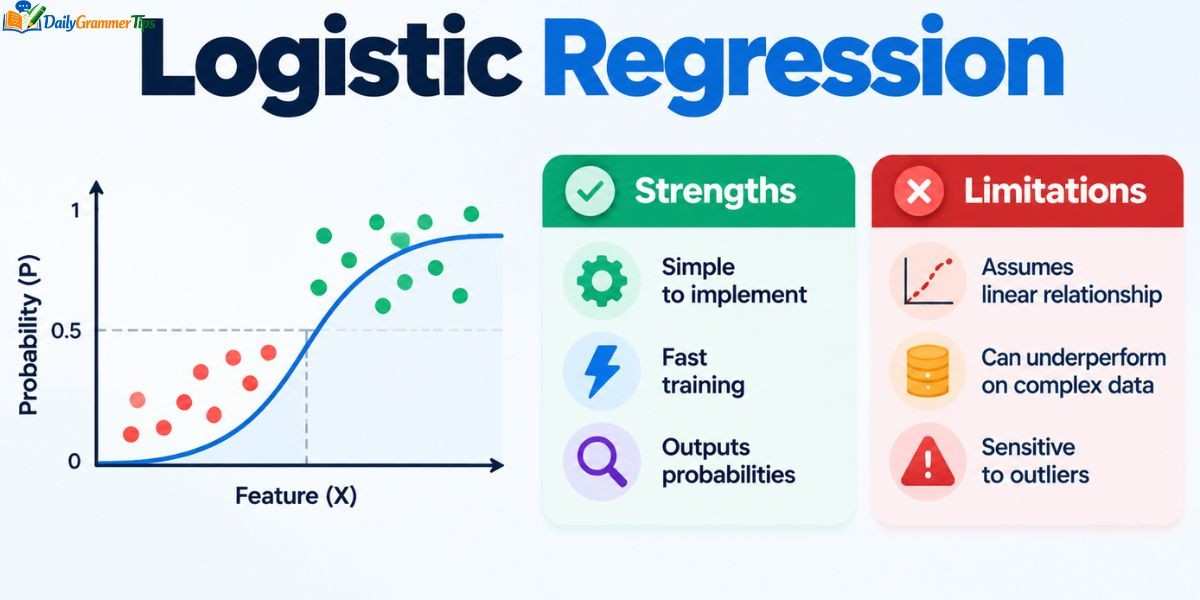
Every tool has trade offs. Here is an honest summary.
Strengths
- It trains fast, even on large tables.
- It gives probabilities, not only labels.
- It offers coefficients that people can interpret.
- It resists overfitting when you add regularization.
- It works well as a baseline for harder problems.
Limits
- It draws a linear boundary, so it struggles with complex patterns.
- It needs careful feature engineering for nonlinear effects.
- It reacts badly to strong multicollinearity.
- It can underperform on image, audio, and raw text data.
- It needs enough examples of the rare class.
When the limits hurt, try tree ensembles, support vector machines, or neural networks. Still, many teams find that a well prepared logistic model comes close to those complex rivals.
Frequently Asked Questions
What is logistic regression in simple terms?
Logistic regression predicts the chance that something belongs to a category, such as spam or not spam. It turns input numbers into a probability between zero and one.
What is logistic vs linear regression?
Linear regression predicts a continuous number, while logistic regression predicts the probability of a class. Linear regression draws a straight line, and logistic regression draws an S shaped curve.
Is logistic regression a form of AI?
Yes, it counts as a basic machine learning method, and machine learning sits inside AI. It learns patterns from data to make predictions.
Can XGBoost be used for logistic regression?
Partly. XGBoost offers a binary logistic objective and a linear booster that mimics the model. Its default tree booster works differently.
When to use logistic regression?
Use it when your target has categories and you want clear, explainable probabilities. It works best on structured data with a roughly linear link to the log odds.
Conclusion
Logistic regression turns a simple idea into a dependable tool. It builds a linear score, passes it through the sigmoid function, and returns a probability. You can read its coefficients, check its assumptions, and explain its decisions to anyone.
You now know the formula, the three main types, and the contrast with linear regression. You saw how to code the model from scratch and how to run it with scikit learn. You also saw how researchers use logistic regression to measure risk and effect sizes.
Start your next classification project with this model. Clean the data, scale the features, and fit the baseline. Measure it with precision, recall, and AUC. If it performs well, you have a fast and transparent solution. If it falls short, you have a solid benchmark to beat.
